Trigonometry Graphs with Octave

Octave is a free and open source scientific computing platform. It is especially suited for mathematical operations and has a simple mechanism to plot the data. Trigonometry visualizations are especially powerful with Octave. This article is about how to plot trigonometry visualizations with Octave.

About Octave

Development of Octave started in 1992 by John W. Eaton. It is largely written in C++ and contains an interpreter of the Octave high level scripting language. The Octave language is mostly compatible with Matlab. Its syntax is matrix-based and supports various data structures and even allows object-oriented programming (OOP). Octave can be run from the command line, but also features a graphical user interface (GUI).

Trigonometric Functions in Octave

Octave covers many trigonometric functions. Most work with radians. But a number of functions also work directly with degrees. If you want to convert from degrees to radians, you can multiply degrees by pi/180.

Thus:

radian = degree * pi/180

A list of all the available trigonometric functions is available at the Octave website.

Plotting Sine

In order to make it more interesting, this simple script plots both the sin(x) and the sin(x*3) in the same graph.

For distinguishing one from the other, I use the black color for sin(x) and red for sin(x*3).

Here is the Octave script that you can enter in the editor or run in the Octave command line:

sine.m

x = -10:0.1:10;
plot (x, sin(x), 'k', x, sin(x*3), 'r')

X defines the range of the values of the graph, from -10 to 10.

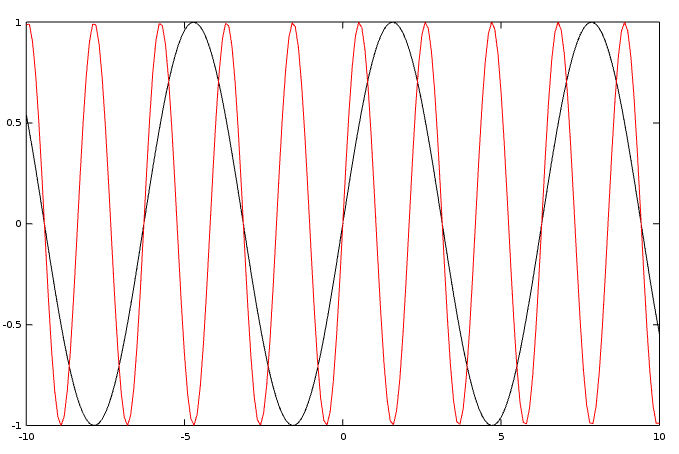
In the graph, you can see that the sin(x*3) has three times the frequency of the sin(x). It is denser packed.

Plotting Sine and Cosine

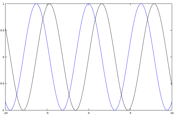
We can also combine a sine and cosine function into one graph. Thus, you are able to see the difference between the two functions clearly.

cosine.m

x = -10:0.1:10;
plot (x, sin(x), 'k', x, cos(x), 'b')

In this case, the sine function is black, and the cosine function is painted blue.

Plotting Tangent

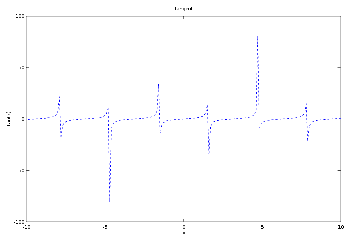
Another interesting function to graph is the tangent function. Tangent is the ratio between sine and cosine.

The only problem with this function is when the cosine becomes zero, because you cannot divide by zero. Thus, whenever the cosine becomes zero it is indicated by asymptotes.

Octave also allows us to add a title and descriptions for the x and y-axis. These are added in the script below:

tan-1.m

x = -10:0.1:10;
plot (x, tan(x), '--')
title('Tangent')
xlabel('x')
ylabel('tan(x)')

The plot for the tangent is dashed, which is due the third parameter of the plot function ('- -').

Be careful not to call your script file name the same as an Octave function because then you get an error.

Conclusion

Writing these little Octave scripts to graph trigonometric functions is not difficult. I hope you got inspired by this article and start exploring the wonders of math on your own.

References

• Octave: https://www.gnu.org/software/octave

Cover photo by vackground.com on Unsplash